HIFI Diary: A Detailed Science Guide on HIFI Cables – The Cable Length Edition

This is an article that was originally meant to be written together with the previous one (the Structure Edition), but considering layout and the specialized nature of the content, I decided it was better to separate them. This installment is a science guide exploring the topic of various cable lengths, primarily aimed at rationally and scientifically investigating the boundaries of cable length. We have often heard in the past that power cables should be as long as possible, and digital cables should be as short as possible. Today, let us discuss together whether these rules of thumb have any actual basis.

Some friends have asked how these cable science guides were written. Here is my unified reply: First, the fundamental concepts of the articles, including the three major cable guides, this Length Edition, and the future Materials Edition, are all a synthesis of my personal experience and accumulated knowledge over the years. However, before putting pen to paper, I used Deepseek and Google/Z-Library to consult some forums and reference literature. Subsequently, I wrote out the basic skeleton, but threw the theorem and formula calculations to the AI—after all, having graduated so many years ago, I have long since returned those fundamentals to my teachers. In any case, the calculation results are more accurate than if I did them manually, and I trust no one will have any objections. Finally, after the draft was completed, I threw it to the AI again for proofreading and formatting. The AI’s formatting looks much better than my own, and so this science guide was produced.

I. Power Cables

The core physical parameter determining the length of a power cable is loop resistance. Current flows through the live and neutral conductors—one out, one back. The total resistance is:

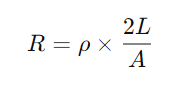
Where:
ρ is the resistivity (for copper, taken as 1.72×10⁻⁸ Ω·m)
L is the cable length (in meters)
A is the cross-sectional area (in m²)
The factor of 2 arises from the two conductors forming the loop.

Voltage drop: ΔU = I × R, where I is the instantaneous peak current.

Inside an amplifier, there is typically a structure consisting of a rectifier bridge and a main filter capacitor. During each half-cycle of AC power, the rectifier bridge conducts only when the forward voltage across it exceeds the diode drop (approximately 1.4V), replenishing the charge in the filter capacitor. The conduction window is very narrow—only for a very short time near the peak of the AC voltage waveform does current flow into the capacitor in the form of sharp pulses.

When the music contains sustained high dynamics (such as drumbeats, strong cello passages), the filter capacitor is rapidly drained by the output stage. If there is a significant voltage drop across the power cable at this moment, the effective voltage present at the input of the rectifier bridge during conduction is reduced, and the capacitor cannot be charged to a sufficiently high voltage within the same window of time. The result is an instantaneous sag in the DC supply rail, limiting the amplifier’s output swing—manifesting audibly as dynamic compression, softened bass, and sluggish transient response.

Engineering data sources for the audibility threshold:

• The professional amplifier design handbook (Audio Power Amplifier Design Handbook) generally holds that when the supply rail voltage drops by more than 2%–3% during peak current draw, most listeners can perceive a loss of dynamics in an A/B comparison.
• More stringent Hi-Fi standards recommend controlling the peak voltage drop of the entire power supply system (including in-wall wiring, sockets, and power cable) to within 1% to ensure transparent transmission.

Converted to the voltage drop of the power cable alone:

Taking 230V AC RMS as an example, the peak voltage is approximately 325V. A 1% voltage drop (calculated based on peak voltage) is about 3.25V. However, since the power cable only accounts for a portion of the entire power supply loop (which also includes in-wall wiring, fuses, socket contact resistance, etc.), the budget allocated to the power cable is typically more conservative: it is recommended to control the peak voltage drop caused by the power cable itself to within 0.5% (corresponding to approximately 1.6V peak drop, or about 1.15V RMS drop). Beyond this value, especially when the voltage drop reaches 1% (about 3.3V peak drop), it easily exceeds the 2% total threshold when superimposed with other parts of the system.

Let us take a high-power power amplifier as an example, drawing an instantaneous current of 15A from the wall outlet at dynamic peaks (already a fairly severe domestic scenario). Calculate the voltage drop as a percentage of the mains RMS voltage:

Cross-Sectional Area	Cable Length	Loop Resistance	Peak Voltage Drop (15A)	Percentage of 230V	Assessment
0.75 mm²	1.5 m	0.0688 Ω	1.03 V	0.45%	Near warning line
0.75 mm²	3.0 m	0.1376 Ω	2.06 V	0.90%	Exceeds standard (approaching 1%)
2.5 mm²	1.5 m	0.0206 Ω	0.31 V	0.13%	Excellent
2.5 mm²	3.0 m	0.0413 Ω	0.62 V	0.27%	Good
4.0 mm²	1.5 m	0.0129 Ω	0.19 V	0.08%	Outstanding
4.0 mm²	3.0 m	0.0258 Ω	0.39 V

Conclusion:

• A 0.75 mm² stock cable is acceptable at 1.5 meters (0.45%), but by 3 meters the voltage drop has reached 0.9%, near the boundary of audibility. For giant power amplifiers with peak current exceeding 15A, even 1.5 meters is a bit tight.
• Cables of 2.5 mm² and above, within 3 meters, all fall well below the 0.5% recommended upper limit, making them completely safe.
• Therefore, for high-current equipment, power cables are recommended to be ≤2 meters in length, with a cross-sectional area of ≥2.5 mm², and 4 mm² is recommended. If a longer distance is unavoidable (e.g., 5 meters), then 6 mm² or larger is required.

An Easily Overlooked Bottleneck: In-Wall Wiring

No matter how much you spend on a 4 mm² or 6 mm² audiophile power cable, the true greatest bottleneck of the entire power supply loop is the segment of in-wall wiring running from the distribution board to your wall socket. Many older houses use 1.5 mm² or 2.5 mm² PVC-insulated wire, and the length may reach 10 meters or even longer. This means the resistance of the in-wall wiring may already be 5 to 10 times that of your power cable.

In other words, while replacing a thick power cable is beneficial, if the in-wall wiring is aged or undersized, the primary contributor to the final voltage drop remains the in-wall section.

• If conditions permit, run a dedicated line (at least 4 mm² or larger) directly from the distribution board to the audio outlet.
• If the in-wall wiring cannot be changed, at least ensure the power cable itself is not overly long or thin, and try to keep the distance from the wall socket to the equipment within 2 meters.

Low-Current Devices (DACs, Digital Interfaces, Preamplifiers)

The peak current for these types of devices is typically <1A. Even if using a 0.75 mm² × 3 m cable, the voltage drop is only about 0.14V (0.06% of 230V), making dynamic compression completely impossible. For low-current devices, length considerations relate almost exclusively to shielding and noise pickup. A well-constructed shielded cable (1.5–2 meters) is more likely to yield a perceptibly blacker background and richer detail than a short but unshielded stock cable.

Special note: power cables are not necessarily “the shorter, the better.” Excessively short power cables often introduce excessive bending or mechanical stress during routing, which is actually detrimental to the plugs, sockets, and the internal structure of the cable itself. However, it should also be known that excessively long power cables, with their own weight, can also place a significant burden on plugs/sockets, potentially leading to deformation over long-term use, causing poor contact and accelerating oxidation. In short, while cable vibration isolation is truly an extremely niche practice, the physical demands underlying it are quite real.

II. Digital Cables — SPDIF Coaxial

In a Hi-Fi system, SPDIF coaxial cables primarily transmit the S/PDIF signal (usually via RCA or BNC connectors) between a CD transport, digital interface, and DAC. Unlike power cables, the length of a coaxial cable is constrained by physical factors acting in two opposite directions:

• Too short: Signal reflections caused by impedance discontinuities return too early, superimposing on the original signal edges and increasing jitter.
• Too long: The skin effect + accumulation of dielectric loss round off the square wave edges, also increasing jitter.

Therefore, SPDIF coaxial cables have a “recommended range”—neither too short nor too long.

Physical Basis for Reflection and Minimum Length

The fundamental frequency of SPDIF is 5.6448 MHz (corresponding to 128 times the 44.1 kHz sampling clock), with a bit period of approximately 177 ns. The propagation velocity of the signal within the cable depends on the Velocity Factor (VF) of the insulating dielectric. Common foamed polyethylene (Foam-PE) coaxial cable has a VF ≈ 0.78, thus the wave speed is:

v = 3×10⁸ × 0.78 = 2.34×10⁸ m/s

When a signal traveling from the transmitter encounters the receiving end or any impedance discontinuity (such as plugs, solder joints, terminal connections), a portion of the energy is reflected back toward the transmitter, then reflected again by the transmitter and arriving at the receiver once more. During this process, reflected energy that overlaps in time with the original signal edge will alter the precise moment the receiver crosses the logic threshold (typically Vref/2), thereby introducing deterministic jitter.

So, how short must a cable be for harmful reflection overlap to occur?

Engineering experience and measured eye diagrams indicate: when the cable length is below 1.2 meters, the round-trip time of the reflected pulse significantly overlaps with the signal rise time (typical value 20–30 ns), the horizontal opening of the eye diagram narrows, and jitter markedly increases. When the cable length reaches 1.5 meters, the round-trip time is approximately 12.8 ns (2 × 1.5 / 2.34e8), which already exceeds the window stabilization time of the PLL in the vast majority of receivers, causing the reflection to fall outside the decision window. This explains why 1.5 meters is widely regarded as the minimum safe length for an SPDIF coaxial cable.

An important clarification: the premise for the above conclusion is that “non-ideal impedance matching exists in the system.” Theoretically, if the characteristic impedance of the transmitter, cable, and receiver are all precisely 75 Ω, and the connectors offer a perfect transition, the reflection coefficient would be zero, and length would no longer pose any constraint whatsoever. But in actual HIFI systems, RCA plugs themselves cannot consistently maintain 75 Ω (BNC is better but still not perfect), and coupled with differences in the output stages of different brands of equipment, reflections will always exist. Therefore, the 1.5-meter rule is a conservative recommendation that balances engineering margin with real-world non-idealities, rather than an absolute physical law.

Physical Basis for Skin Effect and Maximum Length

When a coaxial cable transmits a digital square wave, the attenuation of high-frequency harmonics (at least the 5th harmonic is required to maintain recognizable edges) accumulates with increasing length. Once the edges are rounded to a certain degree, the receiver’s PLL cannot accurately lock onto the zero-crossing point, resulting in additional random jitter. The skin depth formula is:

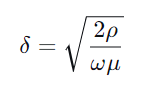
​Where ρ is the resistivity of copper, ω = 2πf, and μ is the magnetic permeability (for copper, close to the vacuum permeability 4π×10⁻⁷). Calculated at 28 MHz (the 5th harmonic), the skin depth is approximately 12.5 μm. For a typical 75 Ω coaxial cable (center conductor diameter approximately 0.8 mm, radius 400 μm), the skin effect causes a substantial reduction in the effective conduction area, and the AC resistance increases significantly.

At the same time, the dielectric loss tangent (tanδ) of the insulating material also increases linearly with frequency. Solid PVC has a tanδ of about 0.02–0.05 at 10 MHz, whereas foamed PE can be as low as below 0.0002. Therefore, the dielectric quality of the cable directly determines the usability for long-distance transmission.

Engineering measurement data:

• High-quality 75 Ω foamed PE coaxial cable (e.g., Belden 1694A): at a length of 10 meters, the insertion loss for the 28 MHz harmonic is about 1.5–2 dB, and the edges can still be maintained steep.
• Common PVC-insulated coaxial cable: at 5 meters, the loss at the same frequency point can reach 3–4 dB, and the eye diagram already appears blurred.
• Beyond 10 meters, even quality cables begin to accumulate noticeable jitter, and the PLL of some DACs may lose lock.

III. Digital Cables — USB

USB is currently one of the most common interfaces for connecting a digital source to a DAC in Hi-Fi systems. USB 2.0 High-Speed mode (480 Mbps) has an extremely high signal frequency, imposing unique requirements on cable length and version selection.

Reflections and Minimum Length: A Protocol-Based Re-examination

USB 2.0 High-Speed signals employ a bit rate of 480 Mbps, with a single bit period of T_bit ≈ 2.08 ns. The signal propagation velocity in the cable is taken as v ≈ 2.1×10⁸ m/s (VF ≈ 0.7). The round-trip time of a reflected pulse, t_round = 2L/v, is calculated as follows:

Cable Length	Round-Trip Time	Ratio Relative to 2.08 ns Bit Period
0.2 m	≈ 1.9 ns	≈ 0.9 × T_bit
0.5 m	≈ 4.8 ns	≈ 2.3 × T_bit
1.0 m	≈ 9.5 ns	≈ 4.6 × T_bit

From a reflection standpoint, even for a 0.2-meter short cable, the round-trip time of a reflection is already close to a full bit period. This means that, under the high-speed handshake and adaptive equalization mechanisms of the USB protocol, short cables will not simply cause jitter the way SPDIF does due to reflected pulses falling within the bit decision window—the USB receiver inherently possesses greater fault tolerance.

USB 2.0 vs USB 3.0: Which Is More Suitable for Audio?

Almost all DACs on the market use the USB 2.0 protocol for audio transmission, even if their physical connector is Type-C or even a USB 3.0 Type-B. This is not a cost issue, but has solid technical reasoning behind it.

USB 2.0’s 480 Mbps bandwidth is sufficient to transmit 32 channels of 192 kHz/24-bit audio. For a domestic two-channel DAC, it does not even use a fraction of that bandwidth. Professional audio manufacturer Focusrite explicitly states on its official support page: “USB 3.0 will not provide lower round-trip latency for audio devices compared to USB 2.0, because latency is determined by the processing cycle of the host driver stack, not the bus speed.” In other words, for audio transmission, USB 3.0’s high bandwidth is “performance overkill.”

Lower Interference, Cleaner USB 2.0

To achieve 5 Gbps high-speed transmission, USB 3.0 introduces technologies such as Spread Spectrum Clocking (SSC) to address EMI, but the electromagnetic interference it generates is itself more complex. Additionally, USB 3.0 cables add multiple high-speed differential signal pairs such as TX/RX compared to USB 2.0, creating the potential for crosstalk between these signal lines. Hi-Fi manufacturers generally believe that USB 2.0 generates less electromagnetic interference than USB 3.0.

Compatibility Considerations

While USB 3.0 interfaces are backward compatible with 2.0 devices, some motherboards’ integrated USB 3.x controllers exhibit compatibility issues when processing USB audio data, which can instead lead to instability such as dropouts or popping noises. This is the pragmatic reason why many DAC manufacturers insist on using purely the USB 2.0 protocol.

IV. Analog Cables — RCA and XLR

Analog audio cables are used to transmit line-level signals after decoding (from a preamplifier) or before the speaker-level signal output by a power amplifier. There are two common connector types: RCA unbalanced (single-ended) and XLR balanced (differential). Their length limits are determined by entirely different physical mechanisms.

RCA Unbalanced Cables: Distributed Capacitance × Output Impedance = Low-Pass Filter

An RCA cable consists of a center signal conductor and an outer shield. Distributed capacitance exists between the signal conductor and the shield (unit length value approximately 50–150 pF/m, with a typical coaxial cable around 100 pF/m). This capacitance, together with the output impedance R_out of the upstream device, forms a first-order RC low-pass filter, with a cutoff frequency of:

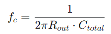
Where C_total = C_per_meter × L, with L being the cable length.

When f_c falls below 20 kHz, high frequencies in the audio band (10 kHz–20 kHz) will experience amplitude attenuation and phase shift. Even if f_c is far above 20 kHz, excessively high distributed capacitance may interact with the instability tendencies of certain amplifiers, causing high-frequency oscillation or transient distortion.

Typical Calculation (using common 100 pF/m cable as an example):

Output Impedance R_out	Cable Length	Total Capacitance C_total	Cutoff Frequency f_c	Effect on Audio
100 Ω (Solid-state preamp)	2 m	200 pF	~8 MHz	Completely transparent
100 Ω (Solid-state preamp)	10 m	1000 pF	~1.6 MHz	Still far above 20 kHz
1 kΩ (Certain tube preamps)	2 m	200 pF	~796 kHz	No effect
1 kΩ (Certain tube preamps)	10 m	1000 pF	~159 kHz	Still outside audio band, but phase shift measurable
10 kΩ (Extremely rare)	5 m	500 pF	~32 kHz	Attenuation already present at 20 kHz

Conclusion: For the vast majority of solid-state output devices (R_out ≤ 200 Ω), an RCA cable within 10 meters will not produce any audible high-frequency attenuation due to distributed capacitance. Only when the output impedance is extremely high (> 5 kΩ) or the cable length exceeds 20 meters may high-frequency roll-off appear. The distance of a few meters in a domestic environment is completely safe.

The True Enemy is Noise: Unbalanced transmission has virtually no ability to reject common-mode interference (such as 50 Hz/60 Hz mains noise radiated from power cords). A long RCA cable acts like a long antenna, making it easier to pick up ambient electromagnetic interference, resulting in an elevated noise floor and AC hum. Therefore, the practical length recommendation for RCA cables is no more than 3–5 meters. If a longer run is necessary, an XLR balanced cable should be used instead.

XLR Balanced Cables: The Length Advantage of Differential Transmission

An XLR balanced cable contains three conductors: positive phase, inverted phase, and an independent shield. The signal is transmitted differentially—the positive and inverted phases carry signals of equal amplitude but opposite polarity. The differential amplifier at the receiving end is sensitive only to the differential-mode signal between the two lines, possessing an inherent ability to cancel common-mode noise appearing simultaneously on both lines (such as external electromagnetic interference), with a Common-Mode Rejection Ratio (CMRR) typically >60 dB.

The main factors limiting length are no longer distributed capacitance, but instead:

• The differential-mode capacitance of the cable (the capacitance between the positive and negative lines, typical value 30–60 pF/m, far smaller than the single-ended line-to-ground capacitance)
• DC resistance (excessive length causes negligible signal level loss, but it is acceptable)
• Cumulative noise pickup by the shield

Calculation: Taking differential-mode capacitance of 50 pF/m and output impedance of 100 Ω as an example:

Cable Length	Total Differential-Mode Capacitance	Cutoff Frequency (Differential-Mode)	Effect on Audio
10 m	500 pF	~32 MHz	None
50 m	2500 pF	~6.4 MHz	None
100 m	5000 pF	~3.2 MHz	Still safe
300 m	15000 pF	~1.1 MHz	Still far above 20 kHz

Professional Audio Practice: In live sound reinforcement and recording studios, XLR balanced cables exceeding 100 meters are routinely used and can still maintain extremely low noise and high fidelity. In the broadcast field, when using high-quality cable (such as Canare L-4E6S, Belden 8412) and isolation transformers, transmission distances can reach over 300 meters.

Conclusion: For home Hi-Fi systems (a few meters to a dozen or so meters), the length of XLR balanced cables is absolutely not a performance bottleneck. The sole reasons to choose XLR are its interference rejection capability and the stability it provides for long-distance transmission, not because RCA cables are inadequate over short distances.